
Every machine learning model revolves around minimizing a cost function, and that minimization is pure calculus. This article covers the core calculus concepts behind ML, with hands-on code in JAX so you can see each idea in action.
JAX is a hardware-accelerated numerical computing library with built-in automatic differentiation. It happens to be a great fit for exploring calculus in an ML context.
Derivatives: Rate of Change
A derivative measures the rate of change of one quantity with respect to another. It’s how we describe change in the real world.
Think about driving a car. You track the distance covered over time. The distance only goes up (you can’t un-drive a road), so you get a monotonically increasing curve:
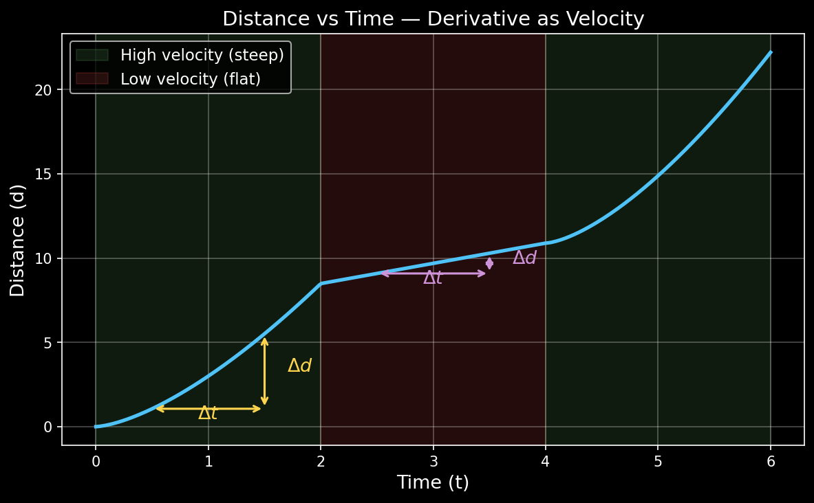
Now look at the curve carefully. Between $t = 0$ and $t = 2$, the car covers a lot of ground — the curve is steep. Between $t = 3$ and $t = 5$, the curve flattens — the car is slower. The steepness of the curve at any point is the velocity, i.e., the rate of change of distance with respect to time.
In any small interval, the rate of change is:
$$\text{velocity} = \frac{\Delta y}{\Delta x} = \frac{\text{change in distance}}{\text{change in time}}$$The derivative is simply this ratio in the limit, as the interval shrinks to zero:
$$f'(x) = \lim_{\Delta x \to 0} \frac{\Delta y}{\Delta x} = \lim_{\Delta x \to 0} \frac{f(x + \Delta x) - f(x)}{\Delta x}$$The Tangent Line and $\tan(\theta)$
How does this connect to geometry? At any point on a curve, the derivative equals the slope of the tangent line at that point. And a slope is just $\tan(\theta)$.
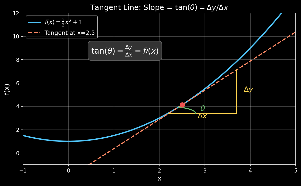
Picture a right triangle formed by the tangent line. The horizontal side is $\Delta x$, the vertical side is $\Delta y$, and $\theta$ is the angle the tangent makes with the horizontal axis. Basic trigonometry gives us:
$$\tan(\theta) = \frac{\Delta y}{\Delta x} = f'(x)$$A steeper tangent (larger $\theta$) means a higher derivative — the function is changing faster. A flat tangent ($\theta = 0$) means the derivative is zero — you’re at a peak, valley, or flat region.
The derivative at a point tells you how steep the curve is there, and gradient descent uses exactly this steepness to decide which direction to step.
Minima and Maxima: Where the Derivative is Zero
If the derivative tells us how steep the curve is, what happens when the steepness is zero? The tangent line goes flat. That means we’re at a point where the function momentarily stops increasing or decreasing — a minimum or a maximum.
$$f'(x) = 0 \implies \text{potential minimum or maximum}$$At a minimum, the function curves upward (like the bottom of a bowl), so the second derivative is positive: $f''(x) > 0$. At a maximum, it curves downward, so $f''(x) < 0$.
This is exactly how optimization works in ML. We have a loss function and we want its minimum. We look for points where the gradient is zero (or close to it), and gradient descent nudges us toward those points step by step.
Finding the Optimal Procurement Split with JAX
Here’s a practical example. Suppose you procure a product from two suppliers, A and B, and you want to minimize cost volatility. Let $\omega$ be the fraction you order from A — the rest comes from B. The blended price is:
$$f(\omega) = \omega \cdot p_A + (1 - \omega) \cdot p_B, \quad \omega \in [0, 1]$$Given historical prices from both suppliers, we want to find the $\omega$ that minimizes the variance of the blended price. That’s a minimum-finding problem, and we can solve it with jax.grad.
import jax
import jax.numpy as jnp

# Historical prices from two suppliers
pA = jnp.array([1408., 1500., 2000., 1800., 1600., 1900., 1700., 1550., 1450., 1650.])
pB = jnp.array([750., 4000., 1500., 3500., 800., 3800., 1200., 3600., 900., 3700.])

def f(w, pA, pB):
    return w * pA + (1 - w) * pB
Evaluating f(w) at any $\omega$ gives a vector of blended historical prices. jax.grad computes derivatives of scalar-valued functions, so we need a scalar loss. A natural choice is the variance of the blended price:
def L(w, pA, pB):
    blended = f(w, pA, pB)
    return jnp.mean((blended - jnp.mean(blended)) ** 2)
Now we compute the gradient of this loss with respect to $\omega$:
dL_dw = jax.grad(L) # derivative of L w.r.t. the first argument (w)
The minimum is where dL_dw is approximately zero. We can scan over a range of $\omega$ values and find it:
w_points = jnp.linspace(0, 1, 1001)
grad_values = jnp.array([dL_dw(w_points[i], pA, pB) for i in range(len(w_points))])

optimal_i = jnp.abs(grad_values).argmin()
optimal_w = w_points[optimal_i]

print(f"Optimal ω = {optimal_w:.3f}")
print(f"Gradient at optimal ω = {dL_dw(optimal_w, pA, pB):.4f}")
print(f"Loss at optimal ω = {L(optimal_w, pA, pB):.2f}")
At the optimal $\omega$, the gradient is near zero — that’s the minimum we were looking for. If $\omega = 0.6$, it means pre-ordering 60% from supplier A and 40% from B gives the most stable blended price across historical data.
Partial Derivatives and Gradients
Real models have many parameters. When $f$ depends on multiple variables, we take partial derivatives: the derivative with respect to one variable while holding everything else constant.
For $f(x, y) = x^2 + 3xy + y^2$:
$$\frac{\partial f}{\partial x} = 2x + 3y, \qquad \frac{\partial f}{\partial y} = 3x + 2y$$The gradient is the vector of all partial derivatives:
$$\nabla f = \left[\frac{\partial f}{\partial x},\ \frac{\partial f}{\partial y}\right]$$It points in the direction of steepest ascent. Gradient descent goes the opposite way.
def f_multi(params):
    x, y = params
    return x**2 + 3*x*y + y**2

grad_f = jax.grad(f_multi)

point = jnp.array([1.0, 2.0])
print(grad_f(point))  # [8.0, 7.0]
# ∂f/∂x = 2(1) + 3(2) = 8 ✓
# ∂f/∂y = 3(1) + 2(2) = 7 ✓
JAX computes the gradient of a scalar-valued function with respect to its first argument. Since we packed x, y into a single array, jax.grad returns the full gradient vector in one call.
Visualizing the Gradient Field
from matplotlib import cm

fig, ax = plt.subplots(figsize=(8, 6))
xs = np.linspace(-3, 3, 30)
ys = np.linspace(-3, 3, 30)
X, Y = np.meshgrid(xs, ys)
Z = X**2 + 3*X*Y + Y**2

# Compute gradient at each point
dX = 2*X + 3*Y
dY = 3*X + 2*Y

ax.contourf(X, Y, Z, levels=20, cmap=cm.coolwarm, alpha=0.7)
ax.quiver(X, Y, -dX, -dY, alpha=0.6)  # negative gradient = descent direction
ax.set_title('Gradient Descent Directions on $f(x,y) = x^2 + 3xy + y^2$')
ax.set_xlabel('x')
ax.set_ylabel('y')
plt.show()
The arrows show the negative gradient, exactly the direction gradient descent would step. They all point toward the minimum.
The Chain Rule: Backbone of Backpropagation
Neural networks are compositions of functions: $L = \ell(g(f(x)))$. To find $\frac{dL}{dx}$, we use the chain rule:
$$\frac{dL}{dx} = \frac{d\ell}{dg} \cdot \frac{dg}{df} \cdot \frac{df}{dx}$$Each layer contributes a local derivative, and we multiply them together. This is what backpropagation does.
Here’s a toy two-layer computation in JAX:
def layer1(x):
    return jnp.tanh(x)

def layer2(x):
    return x ** 2

def composed(x):
    return layer2(layer1(x))

# JAX handles the chain rule automatically
d_composed = jax.grad(composed)

x = 2.0
print(f"composed(x)  = {composed(x):.4f}")
print(f"d/dx composed = {d_composed(x):.4f}")

# Verify manually: d/dx [tanh(x)]² = 2·tanh(x)·sech²(x)
tanh_x = jnp.tanh(x)
sech2_x = 1 - tanh_x**2
manual = 2 * tanh_x * sech2_x
print(f"manual chain  = {manual:.4f}")
Both values match. JAX traces through the entire composition and applies the chain rule automatically, no matter how deep the nesting goes.
Higher-Order Derivatives
Sometimes we care about the curvature of a function, how the slope itself is changing. The second derivative $f''(x)$ tells us this, and it’s central to optimization methods like Newton’s method.
Since jax.grad returns a function, we can differentiate again:
def f(x):
    return jnp.sin(x)

df = jax.grad(f)        # cos(x)
ddf = jax.grad(df)      # -sin(x)
dddf = jax.grad(ddf)    # -cos(x)

x = jnp.pi / 4
print(f"f(x)    = {f(x):.4f}")     # sin(π/4) ≈ 0.7071
print(f"f'(x)   = {df(x):.4f}")    # cos(π/4) ≈ 0.7071
print(f"f''(x)  = {ddf(x):.4f}")   # -sin(π/4) ≈ -0.7071
print(f"f'''(x) = {dddf(x):.4f}")  # -cos(π/4) ≈ -0.7071
In JAX, differentiation operators are first-class, so you can compose them freely.
Gradient Descent from Scratch
Time to implement gradient descent from scratch.
Minimizing a 1D Function
Find the minimum of $f(x) = (x - 3)^2 + 1$. The answer is obviously $x = 3$, but gradient descent should find it on its own:
def loss(x):
    return (x - 3.0)**2 + 1.0

grad_loss = jax.grad(loss)

# Start from a random point
x = 0.0
lr = 0.1  # learning rate
history = [x]

for step in range(50):
    g = grad_loss(x)
    x = x - lr * g
    history.append(x)

print(f"Converged to x = {x:.4f}")  # ≈ 3.0

# Plot the convergence
plt.figure(figsize=(10, 4))
xs = np.linspace(-1, 5, 200)
plt.plot(xs, (xs - 3)**2 + 1, label='$f(x) = (x-3)^2 + 1$')
plt.scatter(history, [(h - 3)**2 + 1 for h in history],
            c=range(len(history)), cmap='viridis', zorder=5, s=20)
plt.colorbar(label='Step')
plt.title('Gradient Descent Converging to the Minimum')
plt.legend()
plt.grid(True)
plt.show()
The dots move from $x=0$ toward $x=3$, slowing down as the gradient gets smaller near the minimum.
Training a Linear Regression
Something closer to real ML: fitting a line $y = wx + b$ to noisy data:
import jax.numpy as jnp
import jax

# Generate synthetic data: y = 2x + 1 + noise
key = jax.random.PRNGKey(42)
x_data = jax.random.normal(key, (100,))
y_data = 2.0 * x_data + 1.0 + 0.1 * jax.random.normal(key, (100,))

def predict(params, x):
    w, b = params
    return w * x + b

def mse_loss(params):
    preds = predict(params, x_data)
    return jnp.mean((preds - y_data) ** 2)

grad_loss = jax.grad(mse_loss)

# Initialize parameters randomly
params = jnp.array([0.0, 0.0])  # [w, b]
lr = 0.1

for step in range(200):
    grads = grad_loss(params)
    params = params - lr * grads
    if step % 50 == 0:
        print(f"Step {step:3d}: w={params[0]:.3f}, b={params[1]:.3f}, "
              f"loss={mse_loss(params):.4f}")

print(f"\nLearned: y = {params[0]:.3f}x + {params[1]:.3f}")
# Expected: y ≈ 2.000x + 1.000
That’s a complete ML training loop in ~15 lines. You write the forward pass, and jax.grad handles the loss gradient for you.
JIT Compilation: Making It Fast
jax.grad handles correctness, and jax.jit handles speed. JIT compiles your Python function into optimized XLA code that runs on CPU/GPU/TPU:
@jax.jit
def training_step(params, lr):
    grads = jax.grad(mse_loss)(params)
    return params - lr * grads

# First call compiles; subsequent calls are blazing fast
params = jnp.array([0.0, 0.0])
for step in range(200):
    params = training_step(params, 0.1)

print(f"Learned: y = {params[0]:.3f}x + {params[1]:.3f}")
For large models, jit provides orders-of-magnitude speedups by fusing operations and eliminating Python overhead.
vmap: Vectorized Gradients
What if you want the gradient of a loss function for each sample individually (per-example gradients)? In pure NumPy you’d write a slow loop. JAX’s vmap vectorizes any function — including gradients:
def single_loss(params, x, y):
    pred = params[0] * x + params[1]
    return (pred - y) ** 2

# Gradient w.r.t. params for a single (x, y) pair
single_grad = jax.grad(single_loss)

# Vectorize over the data dimension — compute per-example gradients
batched_grad = jax.vmap(single_grad, in_axes=(None, 0, 0))

params = jnp.array([0.0, 0.0])
per_example_grads = batched_grad(params, x_data, y_data)

print(f"Per-example gradients shape: {per_example_grads.shape}")
# (100, 2) — one gradient vector per data point

# The mean of per-example gradients equals the batch gradient
print(f"Mean per-example grad: {jnp.mean(per_example_grads, axis=0)}")
print(f"Batch grad:            {jax.grad(mse_loss)(params)}")
vmap is useful for differential privacy (clipping per-example gradients), meta-learning, and Fisher information estimation.
The Jacobian and Hessian
Beyond gradients, JAX provides jax.jacobian for vector-valued functions and jax.hessian for second-order information.
Jacobian
The Jacobian is the matrix of all partial derivatives of a vector-valued function $\mathbf{f}: \mathbb{R}^n \to \mathbb{R}^m$:
$$J_{ij} = \frac{\partial f_i}{\partial x_j}$$def vector_fn(x):
return jnp.array([x[0]**2 + x[1],
x[0] * x[1]**3])
jacobian = jax.jacobian(vector_fn)
x = jnp.array([1.0, 2.0])
J = jacobian(x)
print("Jacobian:")
print(J)
# [[2*x0 1 ] = [[2.0, 1.0],
# [x1^3 3*x0*x1^2]] [8.0, 12.0]]
Hessian
The Hessian is the matrix of second-order partial derivatives — it captures the curvature of a scalar function:
$$H_{ij} = \frac{\partial^2 f}{\partial x_i \partial x_j}$$def scalar_fn(x):
return x[0]**3 + x[0]*x[1]**2 + x[1]**3
hessian = jax.hessian(scalar_fn)
x = jnp.array([1.0, 2.0])
H = hessian(x)
print("Hessian:")
print(H)
# [[6*x0 2*x1 ] = [[6.0, 4.0],
# [2*x1 2*x0+6*x1]] [4.0, 14.0]]
The Hessian tells optimizers like L-BFGS how to take smarter, curvature-aware steps instead of following the gradient blindly.
A Non-Trivial Example: Two-Layer Neural Network
Here we train a tiny neural network on a non-linear function using only JAX primitives:
def relu(x):
    return jnp.maximum(0, x)

def init_params(key, layer_sizes):
    params = []
    for i in range(len(layer_sizes) - 1):
        key, subkey = jax.random.split(key)
        w = jax.random.normal(subkey, (layer_sizes[i], layer_sizes[i+1])) * 0.1
        b = jnp.zeros(layer_sizes[i+1])
        params.append((w, b))
    return params

def forward(params, x):
    for w, b in params[:-1]:
        x = relu(x @ w + b)
    w, b = params[-1]
    return x @ w + b  # no activation on last layer

def loss_fn(params, x, y):
    preds = forward(params, x)
    return jnp.mean((preds - y) ** 2)

# Generate data: y = sin(x)
key = jax.random.PRNGKey(0)
x_train = jax.random.uniform(key, (200, 1), minval=-3, maxval=3)
y_train = jnp.sin(x_train)

# Network: 1 → 32 → 32 → 1
params = init_params(key, [1, 32, 32, 1])

@jax.jit
def step(params, x, y, lr):
    grads = jax.grad(loss_fn)(params, x, y)
    # SGD update — tree_map applies the update to every leaf (weight/bias)
    return jax.tree.map(lambda p, g: p - lr * g, params, grads)

for epoch in range(2000):
    params = step(params, x_train, y_train, 0.01)
    if epoch % 500 == 0:
        print(f"Epoch {epoch}: loss = {loss_fn(params, x_train, y_train):.6f}")

# Plot the result
x_test = jnp.linspace(-3, 3, 200).reshape(-1, 1)
y_pred = forward(params, x_test)

plt.figure(figsize=(8, 5))
plt.plot(x_test, jnp.sin(x_test), label='sin(x)', linewidth=2)
plt.plot(x_test, y_pred, '--', label='Neural net', linewidth=2)
plt.scatter(x_train, y_train, alpha=0.2, s=10, color='gray', label='Training data')
plt.legend()
plt.title('Two-Layer NN Learning sin(x) — Trained with JAX')
plt.grid(True)
plt.show()
jax.grad(loss_fn) applies the chain rule through relu, matrix multiplies, and the MSE loss automatically. jax.tree.map applies the SGD update to every weight and bias in the nested parameter structure. @jax.jit compiles the entire forward + backward + update into a single optimized kernel.
Cheat Sheet: Calculus Concepts → JAX API
| Calculus Concept | Math | JAX |
|---|---|---|
| Derivative | $f'(x)$ | jax.grad(f)(x) |
| Gradient | $\nabla_\theta L$ | jax.grad(loss)(params) |
| Jacobian | $J = \partial \mathbf{f} / \partial \mathbf{x}$ | jax.jacobian(f)(x) |
| Hessian | $H = \partial^2 f / \partial x^2$ | jax.hessian(f)(x) |
| Chain rule | $\frac{dL}{dx} = \frac{dL}{dy}\frac{dy}{dx}$ | Automatic via jax.grad |
| Per-example grad | $\nabla_\theta \ell_i$ | jax.vmap(jax.grad(loss)) |
| JIT compilation | — | jax.jit(fn) |
Conclusion
Calculus isn’t a prerequisite you memorize and forget. It runs inside every training loop. With JAX, you write a Python function, call jax.grad, and the chain rule, partial derivatives, and backpropagation happen for you.
To recap:
- Derivatives measure rate of change, the direction to step.
- Gradients generalize derivatives to multiple parameters.
- The chain rule lets us differentiate through composed functions, i.e. backpropagation.
jax.gradautomates all of this,jax.jitmakes it fast,jax.vmapmakes it parallel.
If you want to understand what your ML framework does under the hood, writing forward passes and letting JAX handle the calculus is a good way to start.
Resources
[1] JAX Documentation — Automatic Differentiation
[2] JAX Quickstart
[3] The Matrix Calculus You Need for Deep Learning — Terence Parr & Jeremy Howard